5. Separating forward and backward waves

The practical use of wave intensity analysis is greatly enhanced by the separation of the measured forward and backward P and U into their forward and backward components. The separation is based on two assumptions: the validity of the water hammer equations and the assumption that the forward and backward waves are additive. Since the water hammer equations follow from the conservation equations for mass and momentum, their validity is equal to the validity of the 1-D equations to describe flow in arteries. The assumption of linearity can be made as accurate as we want by considering smaller and smaller values for dp and du (this is basically the acoustic approximation in gas dynamics). With these assumptions the forward (denoted by subscript +) and backward (denoted by subscript -) pressure changes are

dp₊ = (dp + ρc du)/2
dp_- = (dp - ρc du)/2

The forward and backward velocity changes follow from the water hammer equations

du₊ = dp₊/ρc du)
du_- = - dp_-/ρc du)

If we define the forward and backward wave intensities

dI₊ = dp₊du₊
dI_- = dp_-du_-

they retain the very useful property that dI₊ > 0 and dI_- < 0. Although it is not immediately obvious, it can also be shown that the forward and backward wave intensities add so that

dI = dI₊ + dI_-.

The following script calculates the forward and backward waves.

%% separation of forward and backward waves (ensemble average)
dpep=(dpe + rhoc * due)/2;        % forward pressure difference
dpem=(dpe - rhoc * due)/2;        % backward pressure difference
duep=dpep/rhoc;                   % forward velocity difference
duem=-dpem/rhoc;                  % backward velocity difference
diep=dpep.*duep;                  % forward wave intensity
diem=dpem.*duem;                  % backward wave intensity

pep=cumtrapz(dpep)+pe(1);         % forward pressure waveform
uep=cumtrapz(duep)+ue(1);         % forward velocity waveform
pem=cumtrapz(dpem);               % backward pressure waveform
uem=cumtrapz(duem);               % backward velocity waveform

% figure(50); clf; zoom xon;
% subplot(3,1,1);
% plot(tens,pensavg,'k',tens,pep,'b',tens,pem,'r'),grid on, axis tight;
% ylabel 'Pe-Pd';
% title 'net wave intensity analysis'
% subplot(3,1,2);
% plot(tens,uensavg,'k',tens,uep,'b',tens,uem,'r'),grid on, axis tight;
% ylabel 'Ue';
% subplot(3,1,3);
% plot(tens,die,'k',tens,diep,'b',tens,diem,'r'),grid on, axis tight;
% ylabel 'dIe';
% xlabel 't (s)';

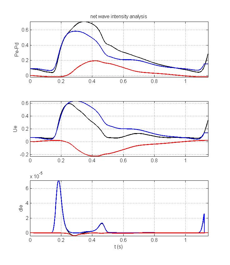
This figure shows the separation of P, U and dI. In each panel the black line corresponds to the measured or net value, the blue line corresponds to the forward component and the red line corresponds to the backward component. In all cases the sum of the blue and red lines is the black line. Note that the forward component of each curve is virtually identical to the measured value, which follows from our assumption that there are only forward waves during early systole. The backward component is delayed, presumably by the time it takes for the forward wave to be reflected back to the site of measurement from the various downstream reflection sites. In the abdominal aorta where these measurements were made, this interpretation is to simplistic because of the possibility of forward waves resulting from re-reflection of backward waves.

For these data, most of the information about the wave intensity can be found in the net wave intensity since the forward and backward waves (denoted by positive and negative values of wave intensity) are fairly distinct. Close inspection of the dI curves around t = 0.25 s, however, shows that the start of the backward wave overlaps the end of the initial compression wave. If the start of the backward wave was taken as dIe = 0, this would result in a slight error compared to the foot of the negative peak in dI_-. In other cases, there can be much more overlap of the forward and backward wave intensity and wave separation is necessary to determine both the magnitude and the timing of forward and backward waves.

There are a couple of technical points that should be mentioned about these results. The forward and backward P and U are determined by 'integrating' the forward and backward pressure and velocity differences. For years we did the integration using the cumsum function in Matlab. A very careful student did the obvious test of comparing the results of this 'integration' to the original signal (i.e. compared P with cumsum(dP)) and found that they could differ by nearly 5%. This is just the numerical error of using sums of differences to calculate an integral. Using the trapezoidal rule reduces the numerical integration error significantly and should be used when integration wave intensity data.

The second point concerns the proper integration constants to use in the integration of the difference data to obtain the measured data. The summing of the forward and backward differences is equivalent to integration and, as with integration, we can added an arbitrary constant to the result. Since the sum of the forward and backward waves must equal the measured wave the sum of the integration constants is determined but there is still a degree of freedom. For example, we can chose the integration constant for the backward waves to be zero and the integration constant for the forward waves to be the measured pressure at t = 0. Alternatively, we can chose both integration constants to be equal so that both the forward and backward pressures are half of the measured pressure at t = 0. Traditionally in the separation of forward and backward waves using impedance methods this is choice that is made; the integration constant for both forward and backward components is defined as half of the mean value of the measured signal. Here, in order to emphasise the correspondence between the forward wave and the measured wave during early systole, we have set the integration constant for the forward waves to be equal to the initial value of the measured wave and the integration constant for the backward wave to be zero.