The first step in wave intensity analysis is to load the relevant data. The location and the structure of the data to be analysed will vary from person to person and application to application. In this case the data that we will analyse is in text format in the subfolder 'data'. We can load it into matlab with the following commands:
%% load data
P=load('..\data\Ao_Pressure.txt');
U=load('..\data\Ao_Velocity.txt');
E=load('..\data\Ao_ECG.txt');
SR=1000;                                % sampling rate
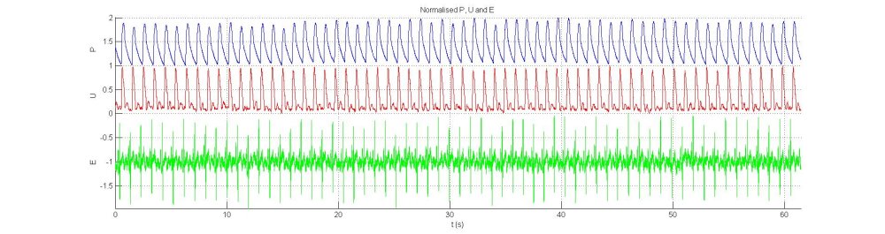
'SR' is the sampling rate which is necessary to convert index values into time. This data was sampled at 1000 Hz. It is essential to examine the data before analysing it to be sure that it is what you think it is. A convenient way to look at all of the data is to normalise it and plot it in the same figure with appropriate offsets. The following code does this and produces the following figure.
%% look at data (scaled)
pp=(P-min(P))/(max(P)-min(P));
uu=U/max(U);
ee=E/max(E);

% figure;
% plot(pp+1),grid on, hold on;
% plot(uu,'r');
% plot(ee-1,'g');
% axis tight;
% ylabel '        E                                 U                      P';
% xlabel 'index'
% zoom xon;
Inspecting the data we see that it is generally of good quality. The ECG trace is rather noisy, but the R-waves are prominent and should be detectable when we get around to ensemble averaging the data. The final matlab command 'zoom xon' is a variant on the normal 'zoom' command that zooms only the x-axis, leaving the scale of the y-axis unaffected. It is very convenient when looking at time series data. Using it to zoom in on the first seven beats, we get the following figure:
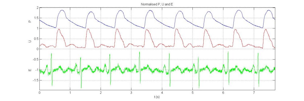
In this view we can see that P is a very regular signal with little noise and the detailed structure of E is clearer than in the unzoomed view. Looking closely at the U signal, we can see that it is pixilated which suggests that the window settings when the data was collected were not optimal. More disturbing, we see that the velocity is unidirectional with no backward velocities during early diastole, which are expected in the abdominal aorta where these data were measured. With the catheter system used to collect these data, there is a choice between unidirectional and bidirectional flow and it could be that the unidirectional option, generally used in the coronary arteries where flow is generally unidirectional, was selected when the data were recorded. We will continue with the data analysis, but this sort of information should be recorded.
It is often useful to look at the frequency content of the data using the fast Fourier transform (FFT). The power spectrum contains useful information about frequencies and hence time scales inherent in the data. The power spectrum of P can be analysed with the following script:
%% power spectrum
fp=fft(P-mean(P));
fu=fft(U-mean(U));
f=(0:N-1)*SR/N;

% figure, grid on, hold on;
% plot(f(1:round(N/2)),abs(fu(1:round(N/2))),'r',f(1:round(N/2)),abs(fp(1:round(N/2))),'b');
% zoom xon;
% xlabel 'f (Hz)';
% ylabel 'power';
% title 'Power spectra of P and U';
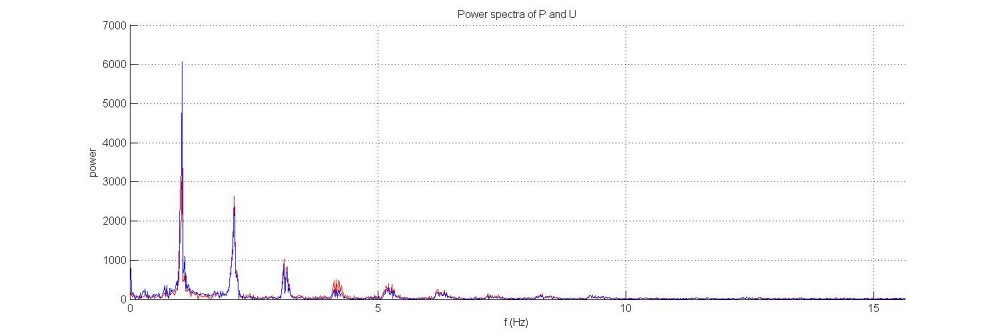
When calculating the power spectrum, it is generally best to subtract the mean of the signal before calculating the FFT. The zero frequency component of the FFT is the mean of the signal and if it is large it can 'spill over' into the lowest frequencies giving an artificial power at the lowest frequencies. The figure shows the FFT of P-mean(P) (blue) and U-mean(U) (red). We see that both spectra are dominated by a large peak at the frequency of the heart beat (slightly greater than 1 Hz for this data) and rapidly decreasing peaks at its harmonics. A very small peak can just be seen at about 0.2 Hz which is generally due to the effect of respiration, and can be much larger in some recordings of arterial pressure.
Another feature apparent from the power spectra is that virtually all of the power is contained in frequencies less than 10-15 Hz. This suggests that these data are over sampled. More useful for further data analysis, this provides us with a way of determining the size of windows that can be used to filter the data without losing significant information. If we take 20 Hz as a conservative upper estimate for the frequency threshold, this corresponds to a time of 0.05 s which corresponds to 50 sample points. Thus, a filter with a frame-size of 50 should not have a significant effect on the information contained in the signal.
Having loaded and inspected the data, we can continue with the calculation of the net wave intensity.