Before carrying out more sophisticated analysis of the data, it is prudent to calculate the net wave intensity dI = dPdU. This parameter corresponds to the sum of the power in the forward waves (always positive) and the backward waves (always negative). It tells us much about the instantaneous, local wave activity and involves very few assumptions other than the validity of using the 1-D conservation equations to describe the mechanics of flow in the distensible arteries.
The variables 'dP' and 'dU' refer to the differences in P and U during one sampling period. If divided by the sampling period they would correspond to the discrete differential operator dP/dt and dU/dt. The wave intensity defined using the differentials rather than the differences may be the best approach when comparing magnitudes of wave intensities taken at different sampling rates. However, there are theoretical advantages in using differences and we will follow the conventions of gas dynamics in this guide.
Wave intensity is defined as the product of two differences. Differencing data inevitably enhances the noise in the signal. Therefore, calculation of wave intensity involves the square of enhanced data. Devising difference algorithms that gave reasonably smooth results was a full-time occupation in the early days of wave intensity analysis. We then discovered Savitsky-Golay filters and they have been an important, almost integral part of wave intensity analysis ever since. They are so important to the analysis that we will provide a detailed description of their implementation. For an excellent, concise description of the theory underlying them refer to Numerical Recipes by Press, Flannery, Teukolsky and Vetterling.
Very briefly, the Savitsky-Golay filter calculates the least squares fit to a polynomial of order N to the data of frame-size F centered on a particular sample time t. Once this polynomial is known it easy to calculate its value at t, and this this value is used for simple smoothing of the data. This can be done very easily using the matlab function 'sgolayfilt'. However, given the fitted polynomial, it is also possible to calculate its derivatives at n, and this is how the filter is used to calculate the smoothed derivative. In order to do this we use the matlab function 'sgolay' in the signal processing toolbox. The syntax is seen in the following example copied from the matlab help material:
N = 4;                 % Order of polynomial fit
F = 21;                % Window length
[b,g] = sgolay(N,F);   % Calculate S-G coefficients
dx = .2;
xLim = 200;
x = 0:dx:xLim-1;
y = 5*sin(0.4*pi*x)+randn(size(x));  % Sinusoid with noise
HalfWin  = ((F+1)/2) -1;
for n = (F+1)/2:996-(F+1)/2,
  % Zero-th derivative (smoothing only)
  SG0(n) =   dot(g(:,1), y(n - HalfWin: n + HalfWin));
  % 1st differential
  SG1(n) =   dot(g(:,2), y(n - HalfWin: n + HalfWin));
  % 2nd differential
  SG2(n) = 2*dot(g(:,3)', y(n - HalfWin: n + HalfWin))';
end
The concept of the filter is ingenious, but the truly inspired idea is their realisation that this process could be carried out quickly and conveniently using normal filter methods by calculating the appropriate filter coefficients ('g' in the above example). The user must decide on the fitting polynomial order, usually N=2 is sufficient for wave intensity analysis (although it might be instructive to try higher polynomial orders) and the frame-size F. This depends on the sampling rate used to measure the data and the time scale over which significant changes are expected in the data. From the discussion in the data inspection section, we will use a frame-size F=51 (the frame-size must be odd). The differences can be calculated using the following script:
%% savitsky-golay differences
Npoly=2;                        % Order of polynomial fit
F=51;                            % Window length
[b,g]=sgolay(Npoly,F);   % Calculate S-G coefficients
HalfWin=((F+1)/2) -1;
p=P-min(P); u=U;         % retain P and U as the original data
dp=zeros(N,1); du=dp; ps=dp; us=dp;
for n=(F+1)/2:N-(F+1)/2
  % Zero-th derivative (smoothing only)
  ps(n)=dot(g(:,1),p(n-HalfWin:n+HalfWin));
  us(n)=dot(g(:,1),u(n-HalfWin:n+HalfWin));
  % 1st differential
  dp(n)=dot(g(:,2),p(n-HalfWin:n+HalfWin));    % pressure difference
  du(n)=dot(g(:,2),u(n-HalfWin:n+HalfWin));    % velocity difference
end
di=dp.*du;                                                      % net wave intensity

% figure(30); clf; zoom xon;
% subplot(3,1,1);
% plot(t,ps),grid on, axis tight;
% ylabel 'P-Pd';
% title 'net wave intensity analysis'
% subplot(3,1,2);
% plot(t,us),grid on, axis tight;
% ylabel 'U';
% subplot(3,1,3);
% plot(t,di),grid on, axis tight;
% ylabel 'dI';
% xlabel 't (s)';
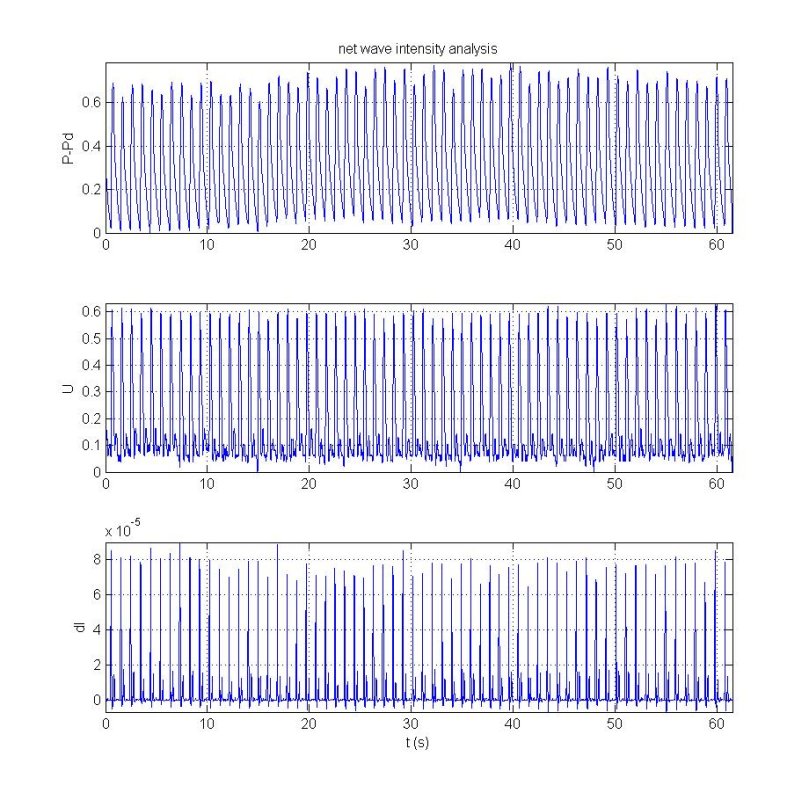
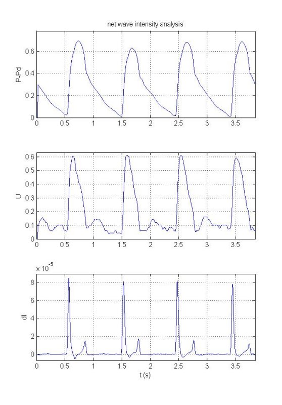
Note that once we have decided on the polynomial order and frame-size we can use the filter coefficients to smooth or difference any of the signals. The result of this script is shown in the following figure where we have used the subplot facility to show the smoothed p, u and di simultaneously:
|
|
The figure on the left shows P-Pd, U and dI for all of the data and in the figure on the left we have zoomed in on the first 3 beats. The pattern of dI is typical of the wave intensity measured in the aorta; a large positive peak at the start of systole (indicating a dominant forward compression wave due to the opening of the aortic valve), a smaller positive peak at the end of systole (indicating a forward expansion wave generated by the relaxation of the ventricle) and a small negative peak during midsystole (indicating the presence of a backward compression wave, probably the result of reflections of the initial forward compression wave). Recall that the sign of dI indicates the direction of the wave (positive for forward and negative for backward). The nature of the waves is determined by looking at the change in the pressure during the wave. If the pressure is increasing, it is a compression wave, and if it is decreasing, it is an expansion wave.
Looking at the very start of the smoothed p and u curves (a similar phenomenon is seen at the end of the data), we see that the differences are zero during a period equal to the half window length. Since the difference cannot be calculated by the filter when the range of the frame is outside of the range of the data, we must make some decision about how to treat that data. One 'pretty' option is to define the smoothed data as NaN's during these intervals so that the plot function simply ignores them. Here, however, we have simply set their values to zero.
The net wave intensity is very simple to calculate and there are very few assumptions in the theory leading to it. This calculation by itself provides interesting clinical and physiological information. If we permit ourselves a few more assumptions, then we can extract even more information about the flow by separating the waves into their forward and backward components. Before we can do that, however, it is useful to introduce the idea of ensemble averaging.