[0. Introduction]
[1. Data Inspection]
[2. Net Wave Intensity]
[3. Ensemble Averaging]
[4. Wave Speed]
[5. Wave Separation]
In the preceding analysis we have calculated the instantaneous wave intensity beat by beat for the whole of the time of measurement. This is vary useful, and a definite strength of wave intensity analysis, when studying dynamic changes to the cardiovascular system. For many applications, however, we are more interest in the 'average' beat rather than the beat by beat variations. The best way to obtain this information is by using the ensemble average.
The ensemble average of a repetitive signal is defined by defining a fiducial time for each beat, creating the ensemble of time varying signals referenced to that time and then averaging across this ensemble at every time throughout the duration of the individual beats. We will use the time of the peak of the R-wave in the ECG as the reference time for each beat in our time series. Other choices are possible and we have used several different reference characteristics of the data to provide the reference times. For example, if ECG data were not measured were not recorded, it is possible to use either the foot of the pressure signal or, preferably in our experience, the time of the maximum dP/dt during the rapid rise in pressure during early systole as the reference time for each beat. In a current project exploring the mechanics of the dicrotic notch, we have found it advantageous to use either the time of the minimum during the dicrotic notch or the time of the minimum dP/dt just prior to the notch as the fiducial times.
The times of the R-waves can be found using many peak detection routines (or, of course, manual selection using the 'ginput' function of matlab). For the following, we will use a program that I wrote many years ago that has proven to be very robust. One common problem that invariably foils this routine is the inversion of the ECG signal caused by switching the electrodes. This is very easily detected by a superficial visual examination of the ECG signal (see the Data inspection section) because all of the R-wave peaks appear as minima. The function that we will use is called Rwave and it returns a vector of the indices at which local maxima occur in the ECG signal (assumed by the function to be the variable E).
%% Rwave.m
% R wave peak detection
% KHP (11/11/08)
%
% assumes the ecg signal is in the variable E
function nb=Rwave(E);
% ns=sampling frequency % nd distance from the first r-wave peak
e=E;
ns=1000;
nd=200;
% find 1st peak
% a=amplitude
% nmax= index corresponding to maximum R-wave peak
[a,nmax]=max(e(1:ns));
j=1;
nb=[];
nb(j)=nmax;
% find rest of the peaks
nend=nb(j)+nd+ns;
while nb(j)+nd+ns < length(e);
    nstart=nb(j)+nd;
    nend=nstart+ns;
    [a,nmax]=max(e(nstart:nend));
    j=j+1;
    nb(j)=nmax+nstart-1;
end
% plot results
% n=1:length(e);
% figure(167);
% plot(n,e,nb,e(nb),'ro');
% axis tight
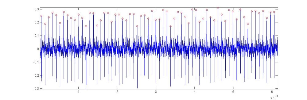
The variable 'ns' in the function is the sampling frequency and it is assumed that the cardiac period is approximately 1 s. The variable 'nd' is essentially a delay time used to ensure that the local maxima are too close to each other. If the algorithm is applied to pathological human data where the heart rate is abnormally high or low, or to animal data where the normal heart rate is not close to 1 Hz, both of these values will have to be adjusted appropriately. When this function is applied to E, the ECG data loaded together with the P and U data, we get the following results
The red circles indicate the peaks that have been found and the indices of these peaks are stored in the vector 'nb'. The figure produced by the function can, of course, be commented out when doing bulk data analysis, but it provides a quick and obvious way to see if the algorithm is performing properly. For these data, the function has found all of the 64 separate heart beats.
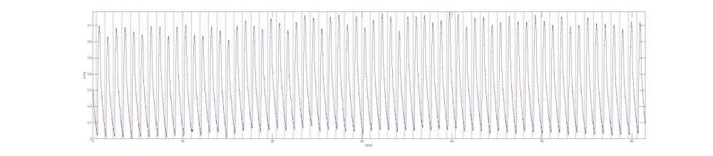
When we transfer the times to the measured P, we get the results shown in the following figure where the dotted red lines correspond to the times of the R-waves on the ECG signal
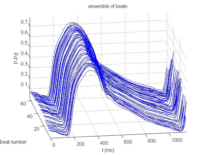
We now create an ensemble of P by forming the matrix pens with dimensions (number of beats X number of times in a beat). It is convenient to use a time period that is slightly larger than the largest cardiac period in the ensemble. This means that some of the data is included twice in the ensemble, once at the start of the beat and again at the very end of the ensemble time. This 'extra' time at the end of the ensemble period gives rise to a rise in pressure at the end of the period as well as the start of the period and gives a useful visual indication of the cardiac period in the ensemble data. This extra time is usually truncated in the final results, but is useful to include it to give a visual indication of the end of diastole. With a little work, the ensemble can be presented graphically as a 3-D plot, as shown in the figure. Each line represents P vs t for a single beat. This format has the advantage that it can be rotated to display the waveforms to advantage. For practical work, however, it is easier to plot the ensemble on a 2-D plot of P vs t. This is equivalent to looking down the beat axis in the 3-D plot. |
|
In Matlab the ensemble average is formed by creating a matrix where successive rows contain the signal relative to successive reference times. In the following script, the length of the ensemble is taken as 1.2 times the average duration of the beats as determined by the difference between successive beats.
%% ensemble average
nb=Rwave(E);                   % returns the indices of the R-wave peaks in the ECG signal
Nb=length(nb);                 % the number of beats detected
nperiod=mean(diff(nb));        % find the average cardiac period
nint=round(1.2*nperiod);       % chose a beat interval slightly longer than nperiod
tens=(0:nint-1)/SR;
pens=zeros(Nb-1,nint);
for n=1:Nb-1
    pens(n,:)=ps(nb(n):nb(n)+nint-1);
    uens(n,:)=us(nb(n):nb(n)+nint-1);
end
pensavg=mean(pens);      % ensemble average pressure
penssd=std(pens);        %    and standard deviation
uensavg=mean(uens);      % ensemble average velocity
uenssd=std(uens);        %    and standard deviation

% figure, grid on, hold on;
% plot(tens,pens');
% plot(tens,pensavg,'k',tens,pensavg+penssd,'k:',tens,pensavg-penssd,'k:','LineWidth',2);
% axis tight;
% ylabel 'P-Pd';
% xlabel 't (s)';
% title 'ensemble average pressure'
% figure, grid on, hold on;
% plot(tens,uens');
% plot(tens,uensavg,'k',tens,uensavg+uenssd,'k:',tens,uensavg-uenssd,'k:','LineWidth',2);
% axis tight;
% ylabel 'U';
% xlabel 't (s)';
% title 'ensemble average velocity'
|
|
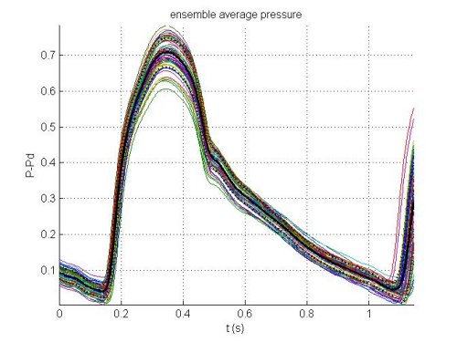
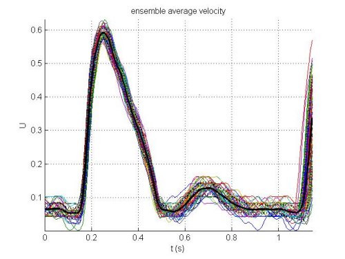
This plot of the ensemble average and the individual members of the average is useful because it is a good indication of the variation in the individual beats making up the ensemble and provides an immediate check for 'outliers' that are generally due to an errant reference time. If outliers are identified, it is easy to remove them from the ensemble and calculate a new ensemble average. Comparing these data to the continuous data previously plotted, it seems that all of the beats are fairly regular and most of the variance comes from the changing mean pressure. The velocity data, on the other hand, exhibit less variation during systole and a lot of variation during diastole when the velocity is small relative to the noise.
We note in passing that except for the calculation of the average beat period, there is no need for the signal to be nearly periodic. Ensemble averaging could equally well be carried out on isolate beats as long as we can identify the appropriate fiducial time for each beat.
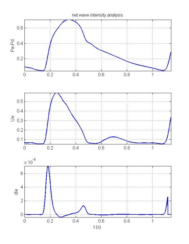
In most of the ensuing analysis we will use the ensemble average data in our calculations. It should be remembered, however, that all of the methods we will discuss are equally valid when applied to instantaneous, beat by beat data. To illustrate this, we now calculate the die, the net wave intensity calculated from the pensavg and uensavg using the follow script
%% wave intensity of the ensemble averages
dpe=zeros(nint,1); due=dpe;
for n=(F+1)/2:nint-(F+1)/2
  % 1st differential
  dpe(n)=dot(g(:,2),pensavg(n-HalfWin:n+HalfWin));    % ensemble average pressure difference
  due(n)=dot(g(:,2),uensavg(n-HalfWin:n+HalfWin));    % ensemble average velocity difference
end
die=dpe.*due;                                         % ensemble average net wave intensity

% figure(40); clf; zoom xon;
% subplot(3,1,1);
% plot(tens,pensavg),grid on, axis tight;
% ylabel 'Pe-Pd';
% title 'net wave intensity analysis'
% subplot(3,1,2);
% plot(tens,uensavg),grid on, axis tight;
% ylabel 'Ue';
% subplot(3,1,3);
% plot(tens,die),grid on, axis tight;
% ylabel 'dIe';
% xlabel 't (s)';
|
Note that the features discussed in the beat by beat analysis are seen in the wave intensity based on the ensemble average data. Because the calculations are nonlinear, it is unlikely that the wave intensity calculated from the ensemble average data will be the same as the ensemble average of the individual wave intensities. We have done a few of these comparisons and generally find that the differences are small compared to the noise in the data. Since we have calculated the standard deviation of the ensemble averages, we have an excellent estimate of the level of noise in the data which we can use to make these comparisons. So far we have calculated only the net wave intensity. This is informative and, because of the small number of assumptions made in its theoretical derivation, a relatively robust measure of wave activity. If we make a few more assumptions it is possible to extract much more data about arterial flow by separating the forward and backward components. Before we can do this, however, it is necessary to determine the local wave speed. |