[0. Introduction]
[1. Data Inspection]
[2. Net Wave Intensity]
[3. Ensemble Averaging]
[4. Wave Speed]
[5. Wave Separation]
4. Estimating local wave speed
The local wave speed plays a very important part in the method of characteristics solution for waves in elastic tubes. The theory tells us that the wave speed is defined by ρ, the density of the fluid (blood), and D, the distensibility of the tube: c=1/(ρ D)1/2. A considerable amount of work has gone into the development and testing of methods of determining c from the measured data. We will discuss and implement two of these methods: a) the PU-loop method and b) the sum of squares method.
b. the PU-loop method
The PU-loop method has become the most frequently used method for determining the local wave speed from the simultaneous measurement of P and U. The theory behind the method are given by the water hammer equations that arise from the method of characteristics solution for flow in an elastic tube. These equations relate the difference in pressure to the difference in velocity across a wavefront. For forward waves (denoted by a + subscript)
dp+ = + ρc du+
and for backward waves (denoted by a - subscript)
dp- = - ρc du-
The first equation says that during periods when there were only forward waves in in the artery a plot of p vs u will be linear with slope equal to ρ c. Since the results of the net wave intensity calculation show that forward waves are dominant during the early part of systole, we can expect the PU=loop to be linear during that period of the cardiac cycle.
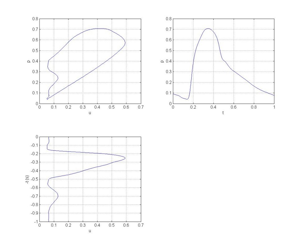
The PU-loop plots P at each sampling time against the U at the corresponding time, as shown in the figure. Since time is simply a parameter in the plot, it is sometimes useful to plot P vs t and U vs t so that they share the P and U axes. By looking at the changes in time of P and U we can easily determine relevant points on the PU loop. For example, in this example measured in the abdominal aorta (and most non-coronary arteries) the end of diastole corresponds to the lower left 'corner' of the loop. The rapid rise in P and U during early systole corresponds to the lower part of the loop. The time of peak U corresponds to the rightmost point on the loop and the time of peak P corresponds to the topmost point. Late systole corresponds to the upper part of the PU-loop. Diastole, when P falls steadily and U is minimal corresponds to the left side of the PU-loop. Thus, we traverse the loop in the counter-clockwise direction as time progresses through the cardiac period. |
|
temporal alignment of data
Wave intensity analysis can be very sensitive to differences in the time delays in the measurements of P and U. These can arise from a number of sources. Delays are usually built into the electronic filtering and processing of the transducer signals, for example the time needed to process ultrasound data is different from the time needed to process data obtained with a strain gauge. Sometimes the sites of the measurements cannot be aligned exactly because of interference between the transducers, for example a pressure catheter within the measurement volume of a Transonic flow meter will corrupt the measurement of flow. Delays due to hardware and electronic circuitry can be measured in in-vitro but the alignment of transducers can be difficult in-vivo. Since a misalignment of 1 cm causes a temporal delay of 1 ms if the wave speed is 10 m/s, these time delays can be significant depending on the modality of the measurements used in wave intensity analysis.
Ideally, delays in the measurements should be calibrated in-vitro and corrected before the start of wave intensity analysis. This has been done in the 8 ms shift applied to the U data in the previous examples. If these calibrations are not available, the PU-loop and the assumption that there are only forward waves during the early part of systole provides a way of aligning the P and U measurements in time.
This is illustrated in the following figure which shows the PU-loop obtained from the ensemble averages pe and ue obtained for our sample data with different shifts in time.
|
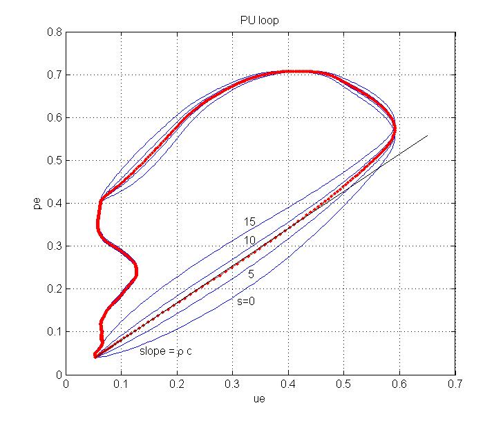
This is illustrated in this figure which shows the PU-loop obtained from the ensemble averages pe and ue obtained for our sample data with different shifts in time. The lower curve labelled s=0 shows the original data as obtained from the measurement system. The portion of the loop corresponding to the initial part of systole is the lower part of the loop when both the velocity and the pressure are increasing. It is clear that this part of the loop is convex rather than linear which is not consistent with the assumption of only forward waves during the early part of systole. The other curves in blue show the loops obtained by shifting the velocity data relative to the pressure data by s=5, 10 and 15 ms. We see that the part of the loop becomes progressively less convex and ultimately concave to the x-axis at the larger shifts. The red curve is for the shift s=8 ms and it produces the most linear result in early systole of any shift (in steps of the sampling time, 1 ms). The thin black line is the linear fit to the early part of the PU-loop for s=8 and its slope is equal to ρc. The dots on the red curve correspond to data points and give a good indication of time and the rate of change observed during different parts of cardiac cycle; the larger separation of the data points indicate that the data are changing much more rapidly during early systole.
This temporal correction of the data is based on the assumption that there are only forward waves during early systole. This may not be true and it is difficult to know a priori when backward waves due to reflections become important at any particular measurement site. In the extreme case of the coronary arteries when backward waves are caused by contraction of the myocardium surrounding the distal vasculature, it is difficult to find any part of the PU-loop that is linear. In cases like this, it is necessary to use another method to estimate the local wave speed, as discussed below.
A considerable amount of effort has gone into the best way of determining the part of the PU-loop that should be used in the determination of wave speed. Least squares comparisons, Baysian inference and other statistical tests have been tried but most researchers some variation of 'fitting by eye' in the calculation of wave speed. This is an area of wave intensity analysis that would benefit from more research. |
If the slope of the PU-loop is linear during early systole, the estimation of the local wave speed is simple. According to the water hammer equation of forward waves the slope of the linear portion of the curve (when there are only forward waves) is equal to ρc. Since ρ, the density of blood, is virtually constant, changing by only a fraction of a percent over the most extreme cases, the wave speed is
c = 1/ρ dP/dU
If SI units are used, P in Pa, U in m/s and ρ in kg/m3, c will be in m/s. Other units will require appropriate scaling. For wave intensity analysis, it is convenient to observe that it is the factor ρc that is needed in the calculations and this can be obtained in whatever unit are used for P and U simply from the slope of the linear portion of the PU-loop. This is useful for calculations, but SI should be used when reporting results.
b. the sum of squares method
The PU-loop method for estimating wave speed cannot be used in cases, such as data from the coronary arteries, where there is no period during the cardiac cycle when backward waves are not significant. Fortunately, theory gives another estimate of wave speed which we refer to as the sum of squares method:
ρc=(Σ dp2/Σ du2)1/2
where the sums must be taken over the entire cardiac period. The theory leading to this estimate assumes that P and U are periodic and that the correlation between the forward and backward changes in velocity is zero; i.e. the integral of du+du- over a cardiac period is zero. Since we believe that most backward waves are reflections of the forward waves, the validity of this assumption is not immediately obvious. However, if there are many reflection sites with different reflection coefficients and delay times, it is possible that this correlation is small.
conclusions
Determination of ρc using the PU-loop method and interactive determination of the part of the loop that is linear can be done with the following script.
%% PU loop
pe=pensavg(1:1000);        % truncate the ensemble average to a period of 1 s
ue=uensavg(1:1000);
te=tens(1:1000);
figure(50); clf;
plot(ue,pe), hold on, grid on;

%% determination of wave speed from PU-loop
a=ginput(2);                    % lower and upper limits of linear portion of the curve
rhoc=(a(2,2)-a(1,2))/(a(2,1)-a(1,1));    % the slope = the product rho x c

% plot(a(1,1),a(1,2),'ro',a(2,1),a(2,2),'ro');
% plot([a(1,1) a(2,1)],[a(1,2) a(2,2)],'r');
% ylabel 'pe';
% xlabel 'ue';
% title 'PU-loop determination of wave speed';
% gtext 'slope = \rho c';
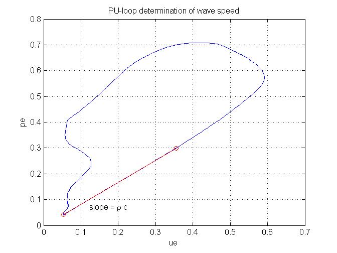
This figure illustrates the determination of ρc using the PU-loop method using the ginput function to chose the portion of the loop that is linear. The blue line is the PU-loop using the ensemble averaged P and U. The red circles indicate the position of the start and end of the linear portion of the loop determined interactively using the ginput function. The red line between the circles is the linear line used to determine the slope and hence the value of ρc. |
|
Studies comparing different estimates of wave speed from measurements of P and U generally show that there is a systematic difference between the results of the different methods. Without an independent way of determining local wave speed (remember that measurement of wave speed by the foot-to-foot method gives an average wave speed over the distance between measurement sites) we still do not know which estimate is the best. Most studies have used the PU-loop method and I would recommend it as the first method to try. When this method cannot be used, I would recommend the sum of squares method.
As we will see in the next section, the estimation of ρc is integral to the separation of forward and backward waves.